Split Testing for Geniuses

You are sitting at a slot machine with two levers, labeled A and B. When you pull a lever, sometimes a dollar comes out of the slot and sometimes not. The casino tells you that each lever has a fixed chance of giving you a dollar (its success rate) but, of course, they don’t tell you what it is. Since you don’t have any way of distinguishing them to start, you pull lever A and a dollar comes out (Yipee!). What do you do next?

Warning! We’ve made some key assumptions here (the success rate is fixed, and the choices are fixed), that will affect our Analysis below. Failing to notice these assumptions has led some very smart people to make some very stupid arguments about Split Testing. Don’t fall into this trap! See the Conclusion for more.

The Strategies

So, did you decide? Do you pull A or B next? What then?

The answer is not so simple. But, you wrack your brain and come up with three strategies you think might work well. Amazingly, these are three of the most used Split Testing strategies (you are a genius, afterall). Let’s explore these strategies, together with implementations in Python, before you choose the best one.

1. Random

The first strategy you come up with is to flip a coin and choose A if the coin comes up heads, and B if it is tails. While simplistic, this is not a bad strategy. It is very simple and very fast. It also does a good job at minimizing our regret; we will choose the best lever around half the time.

This is the Random (aka. Uniform) strategy. You implement it without batting an eye:

import random

def random_strategy(N, n):
    return random.randint(0, 1)

In Python, you are using 0 and 1 to represent levers A and B. The parameters N and n are unused for now. You’ll see their use below.

2. Epsilon Greedy

As you are pulling levers randomly, you noticed that A has been successful on 7/10 pulls, and B on 4/10. You start to suspect that A has a higher success rate than B, and feel like a chump continuing to flip that coin. You are greedy, and want to start pulling A more often.

But how much more often? Sure, you could pull A 100% of the time. But you’re no dummy. You know that hot streaks can easily happen by random chance. There’s a decent chance that B actually has a higher success rate than A, but you’d never figure that out because you’re always pulling A!

Instead, you come up with a better strategy. First you roll a die. If you roll a 1, you then flip a coin to choose a random lever. If you roll anything else, then you choose the lever that has been performed the best so far (earnings per pull).

This is an Epsilon Greedy strategy (with \(\epsilon = \frac{5}{6}\)). In general, Epsilon Greedy algorithms let you choose how “greedy” you want to be (how often you choose the current best performer), by choosing \(\epsilon\). They are also very simple to implement and fast to run.

Note: To determine the “best lever” after a number of pulls, you need to keep track of the number of pulls and dollars for each lever, so get out a pen and paper. In Python, we’ll use a tuple N to keep track of the total number of pulls for each lever, and a tuple n for the number of dollars earned.

You have no trouble implementing this strategy in Python:

import numpy as np

def epsilon_greedy_strategy(N, n, epsilon=5./6):
    if np.all(N > 0) and random.random() < epsilon:
        # Choose the currently best performing option.
        return np.argmax(n / N)
    else:
        # Choose a random option.
        return random.randint(0, 1)

3. Bayesian Bandit

Suddenly, you remember your (too distant!) statistics training. Isn’t this what Bayesian Inference was all about?!

You’re onto something. In Bayesian Inference we declare our prior beliefs about the world, and then update those beliefs as new evidence comes in. Bayes’ theorem tells us exactly how we should update our beliefs given new evidence.

First you have to decide what your prior beliefs are. If you denote the real probability of getting a dollar when you pull lever A as \(p_A\), then your prior belief, \(P_A(\theta)\), is the probability distribution that reflects your current belief about the likelihood that \(p_A = \theta\). Likewise, \(p_B\) and \(P_B(\theta)\) represent lever B. If you haven’t touched either lever, you don’t really have any information to go on: it is equally likely that either lever never gives any dollars, or always, or anything in between. You know nothing. Therefore, you choose your priors to be uniform distributions (equal likelyhood of being anything between 0 and 1).

Now, every time you pull a lever, you learn something about the world, and Bayes’ theorem describes how you should update your beliefs about \(p_A\) and \(p_B\) (these are often called your posterior distributions). You do a little research, and a little math, and are surprised to find that there is a very simple equation that describes what your posterior distribution for a lever will be after showing it \(N\) times with \(n\) successes:

\[P(\theta) = f_{1 + n, 1 + N - n}(\theta)\]

where \(f\) is the Beta distribution.

Excellent! That will make the implementation relatively simple. Your strategy is as follows. After every pull, you will update your posterior belief distributions to reflect what you learned. Then you’ll choose the next lever to pull in accordance with your confidence that it is the best. To do this, you’ll choose a sample success rate from each posterior distribution, and pick the lever that has the highest sampled success rate.

This is the Bayesian Bandit strategy. You sweated a little getting the math and code right, but the result is quite eloquent:

from scipy.stats import beta

def bayesian_bandit_strategy(N, n):
    # Compute a probability distribution representing our current belief
    # about the success rate of each option, based on the evidence in
    # `N` and `n`.
    distributions = [beta(1 + n[i], 1 + N[i] - n[i]) for i in range(2)]

    # Draw a sample success rate from each of our distributions.
    sampled_rates = [dist.rvs() for dist in distributions]

    # Choose the lever with the highest sampled success rate.
    return np.argmax(sampled_rates)

Analysis

Which strategy should you choose? Your success metric is straight-forward: the more money earned, the better. Now, you could simply play the slot machine for a while using each strategy, and count your earnings. You know that might take a while, though. As in many games of chance, a poor strategy here could beat a superior one over the short run.

Instead, you whip out your laptop again and write some code to simulate the slot machine. It’s not so difficult. First, you need to decide on the success rates to use in your simulation, since you don’t know the actual ones. You (somewhat arbitrarily) pick \(p_a = .6\) and \(p_b = .4\), and make a mental note to try other values later to see if the results differ. Then, you simulate pulling the lever 1000 times for each strategy, and add up the number of dollars earned. You notice that the results are a little noisy, so you repeat the simulation 1000 times and compare the average number of dollars earned.

NUM_SAMPLES = 1000
NUM_PULLS = 1000
P = np.array([.6, .4]) # Success rates for each lever.

strategies = [('Random', random_strategy),
              ('Epsilon Greedy', epsilon_greedy_strategy),
              ('Bayesian Bandit', bayesian_bandit_strategy)]

data = []

for _ in range(NUM_SAMPLES):
    for (strategy, choose_lever) in strategies:

        N = np.array([0, 0]) # Number of pulls of each lever.
        n = np.array([0, 0]) # Dollars earned for each lever.

        for pull in range(NUM_PULLS):
            # Decide which lever to pull based on strategy.
            lever = choose_lever(N, n)
            # Count a pull for this lever.
            N[lever] += 1
            # Count a dollar for this lever if successful.
            if random.random() < P[lever]:
                n[lever] += 1
            # Add up the dollars earned so far.
            dollars_earned = np.sum(n)
            data.append([strategy, pull, dollars_earned])

Then you plot the dollars earned per pull.

from ggplot import *
import pandas as pd

# Compile the data into a dataframe for easy plotting.
df = pd.DataFrame(data, columns=['strategy', 'pull', 'dollars'])
# Compute the dollars earned per pull.
df['dollars_per_pull'] = df['dollars'] / (df['pull'] + 1)
# Plot the dollars earned per pull.
p = ggplot(aes(x='pull', y='dollars_per_pull', color='strategy'), data=df) + stat_smooth(span=.1, se=False, size=3) + xlab('Pull') + ylab('Dollars per Pull')
print(p)

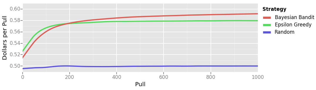
You find that Bayesian Bandit is the best of your three strategies. In the first few pulls, it performs similarly to the Random strategy, but it quickly “learns” that lever A is best and starts pulling it almost exclusively. This is evident in the gradual increase in Dollars per Pull. Note that the best we could expect any strategy to earn is $0.6 per pull, Bayesian Bandit approaches that ideal as we pull more and more.

You also notice that your Epsilon Greedy strategy exhibits a similar rise in Dollars per Pull as it, too, “learns” the best lever. The rise is slower, however, and never passes about $0.58, since we will never choose B on less than 1 of 12 pulls, on average.

The Random strategy, predictably, performs less well than the others. It consistantly earns the average of \(p_A\) and \(p_B\): $0.5.

So you go on happily pulling levers throughout the night using Bayesian Bandit, confident that you’re using a solid strategy.

Conclusion

The implications of this story extend much further than the casino. The question of “which lever to pull” is also known as a Split Testing Strategy . These strategies are used by online ad networks to decide which advertisement to show viewers, by websites to decide which version of a page to show, and many other places. They are widely used, widely discussed, and widely miss-understood.

Have we finally laid the issue to rest, and proven that you should always use Baysesian Bandit, and let Random (A/B) testing go the way of the dodo?

The answer is emphatically no! We made two key assumptions in this story, one explicit and one implicit. First, we assumed that each lever’s success rate is fixed (that is, it doesn’t change over time). Second, we implicity assumed that our slot machine does not get any levers added or removed from it while we are playing. These assumptions are perfectly reasonable when you’re talking about a slot machine, but they might not hold for whatever problem you are actually applying them to. Consider the case of an ad network: the success rate of an ad can easily change seasonally or for many other reasons. It’s also common to add or remove advertisements (aka. levers) into a test at any time. When these assumptions hold, Bayesian Bandit will beat Random over the long run. When they break down, the best strategy is less obvious—there will be trade-offs. And that is a discussion for another post. Stay tuned…